Comparison with other tools#

This document compares OpenBox with other popular black-box optimization (BBO) systems.

Capabilities#

System/Package	FIOC	Multi-obj.	Constraint	History	Distributed	Parallel	Visualization	Algorithm Selection	Ask-and-Tell
Hyperopt	√	×	×	×	√	√	×	√	√
Spearmint	×	×	√	×	×	√	×	√	×
SMAC3	√	√	×	×	×	√	△	×	√
BoTorch	×	√	√	×	×	√	△	×	×
Ax	√	√	√	×	√	√	√	√	×
Optuna	√	√	√	×	√	√	√	×	√
GPflowOPT	×	√	√	×	×	×	×	×	×
HyperMapper	√	√	√	×	×	×	×	×	×
HpBandSter	√	×	×	×	√	√	√	×	×
Syne Tune	√	√	√	√	√	√	√	×	×
Vizier	√	×	△	△	√	√	×	×	×
OpenBox	√	√	√	√	√	√	√	√	√

FIOC: Support different input variable types, including Float, Integer, Ordinal and Categorical.
Multi-obj.: Support optimizing multiple objectives.
Constraint: Support inequality constraints.
History: Support injecting prior knowledge from previous tasks into the current search (i.e. transfer learning).
Distributed: Support parallel evaluations in a distributed environment.
Parallel: Support parallel evaluations on a single machine.
Visualization: Support visualizing the optimization process.
Algorithm Selection: Support automatic algorithm selection.
Ask-and-Tell: Support the ask-and-tell interface.
△ means the system cannot support it for general cases or requires additional dependencies.

Performance#

Experiment setup:

Algorithm selection: The algorithm used in OpenBox is selected via automatic algorithm selection mechanism. For other systems, the algorithm is selected according to the documentation or the default algorithm is used.
Each experiment is repeated 10 times. The mean and standard deviation are computed for visualization.

Constrained Multi-objective Problems#



(a) CONSTR	(b) SRN

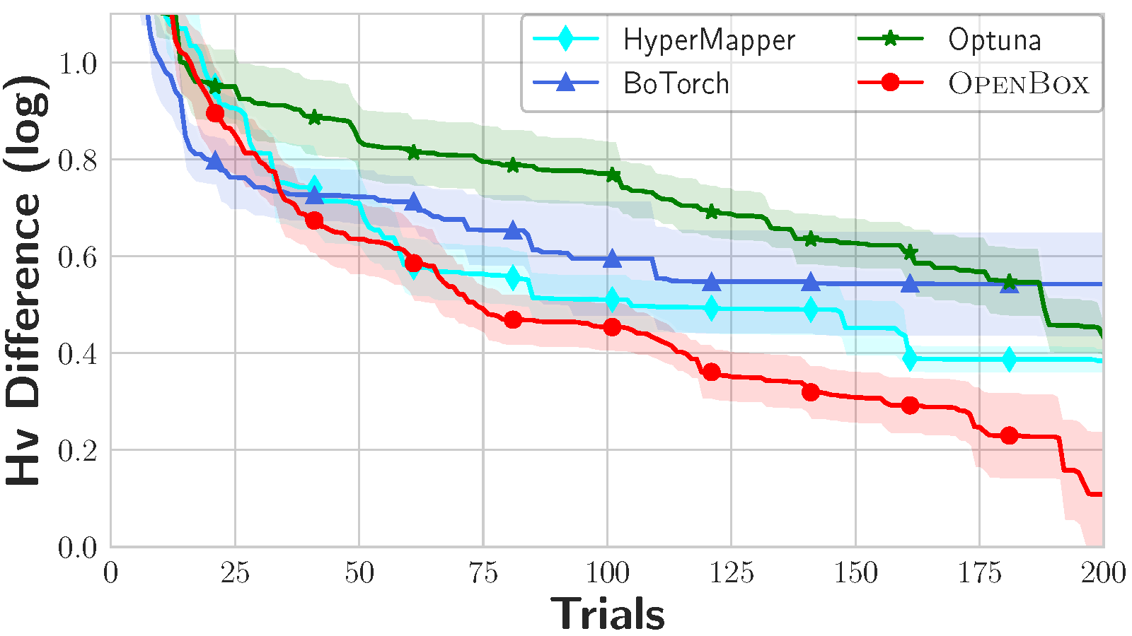
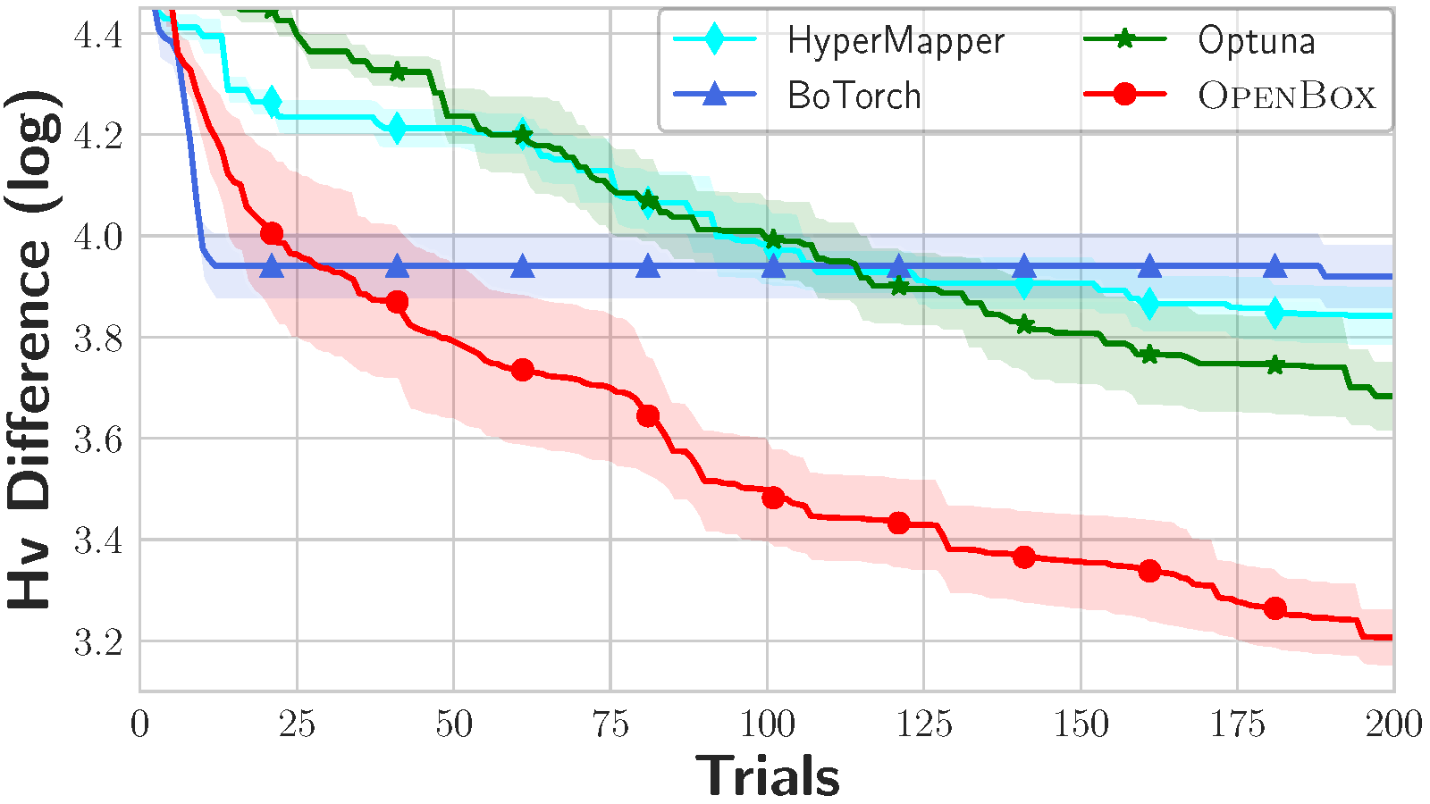
Figure 1: Constrained multi-objective problems.

Setup:

Problems: synthetic functions CONSTR (2 objectives, 2 constraints) and SRN (2 objectives, 2 constraints).
Budget: 200 iterations.
Metrics: Hypervolume difference is the difference between the hypervolume of the ideal Pareto front and that of the estimated Pareto front by a given algorithm.
Algorithm in OpenBox: Gaussian Process with Expected Hypervolume Improvement (auto-selected).

We benchmark the performance of OpenBox on constrained multi-objective problems CONSTR and SRN. As shown in Figure 1, OpenBox outperforms the other baselines on the constrained multi-objective problems in terms of convergence speed and stability.

LightGBM Tuning Task#

Figure 2: LightGBM tuning task.

Table 2: The search space of LightGBM.

Hyper-parameter	Type	Range
n_estimators	integer	[100, 1000]
num_leaves	integer	[31, 2047]
learning_rate	float (log)	[0.001, 0.3]
min_child_samples	integer	[5, 30]
subsample	float	[0.7, 1.0]
colsample_bytree	float	[0.7, 1.0]

Setup:

Problem: tuning LightGBM on 25 OpenML datasets.
Budget: 50 iterations each.
Metrics: Performance rank of the best achieved accuracy among all baselines on each dataset.
Algorithm in OpenBox: Gaussian Process with Expected Improvement (auto-selected).
Algorithm in other systems: Selected based on their documentation or default choice. Please note that the other components in each system, such as the initial design and acquisition function optimizer, can also affect the results.
- BoTorch: Gaussian process (gpytorch) with EI.
- GPflowOpt: Gaussian process (GPflow) with EI.
- Spearmint: Gaussian process with EI.
- HyperMapper: random forest with EI.
- SMAC: random forest with log EI.
- Hyperopt: TPE algorithm.
24 datasets with OpenML id: abalone (183), ailerons (734), analcatdata_supreme (728), bank32nh (833), cpu_act (761), delta_ailerons (803), delta_elevators (819), kc1 (1067), kin8nm (807), mammography (310), mc1 (1056), optdigits (28), pendigits (32), phoneme (1489), pollen (871), puma32H (752), puma8NH (816), quake (772), satimage (182), segment (36), sick (38), space_ga (737), spambase (44), wind (847).

We benchmark the performance of OpenBox on a LightGBM tuning task. Figure 2 shows the box plot of the performance rank of each baseline. The performance rank is the rank of the best achieved accuracy on each dataset. We observe that OpenBox outperforms the other competitive systems, achieves a median rank of 1.25 and ranks the first in 12 out of 24 datasets.

Scalability Experiment on Input Dimensions#



(a) 4d-Ackley	(b) 8d-Ackley

(c) 16d-Ackley	(d) 32d-Ackley

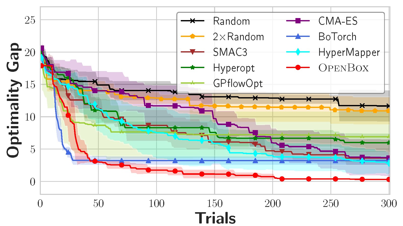
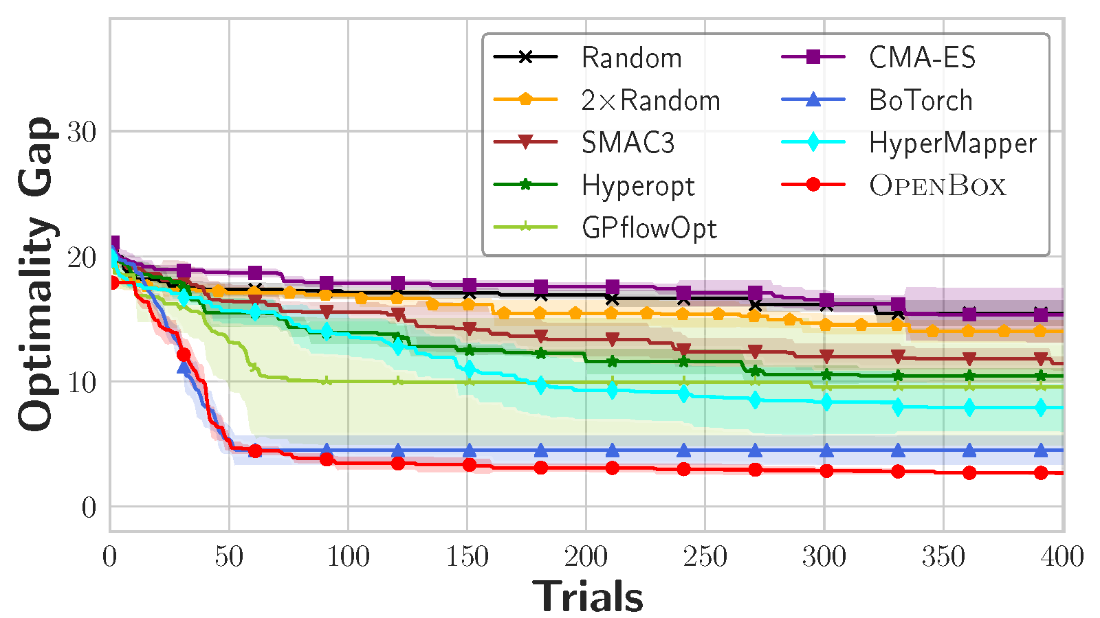
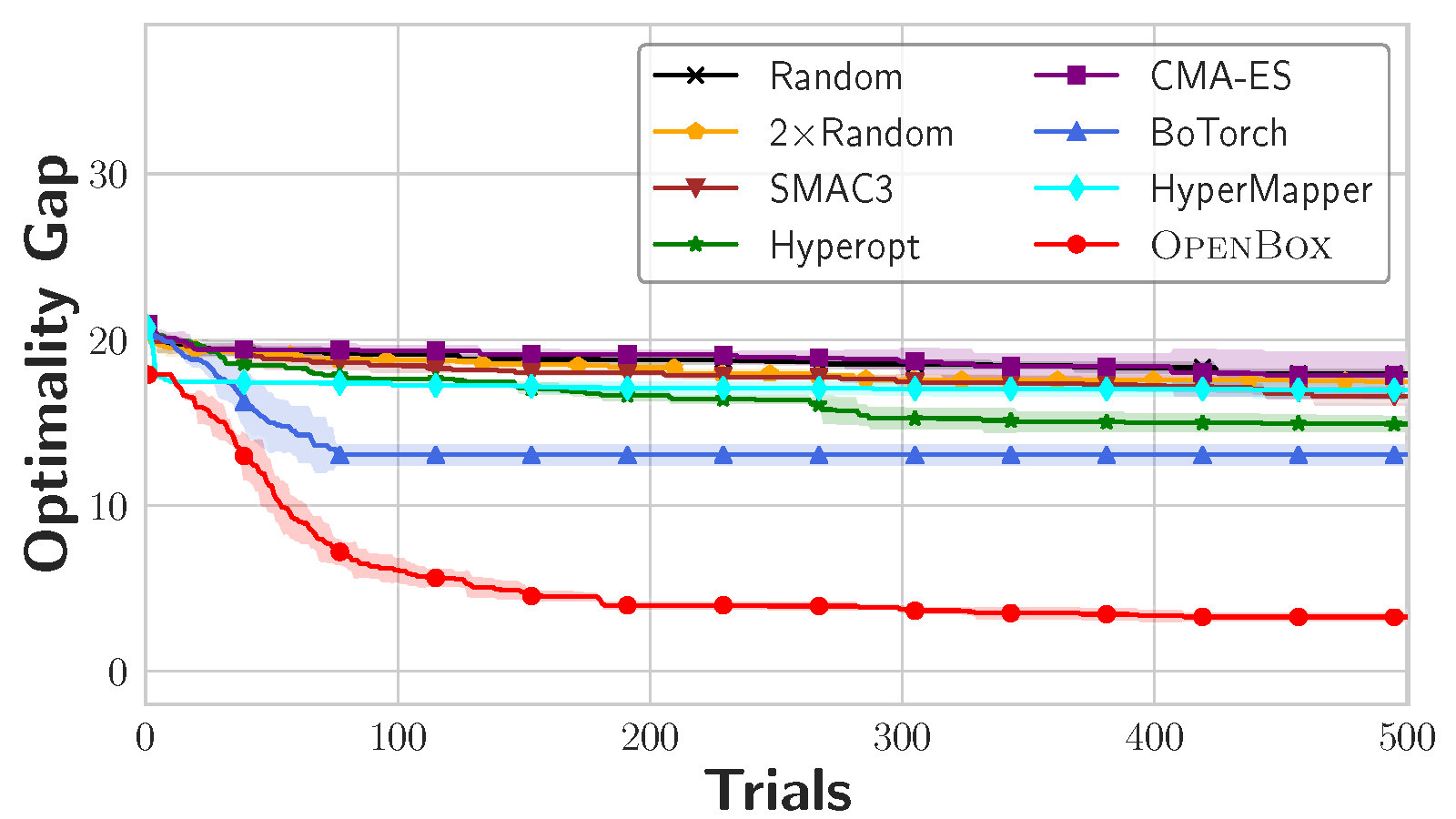
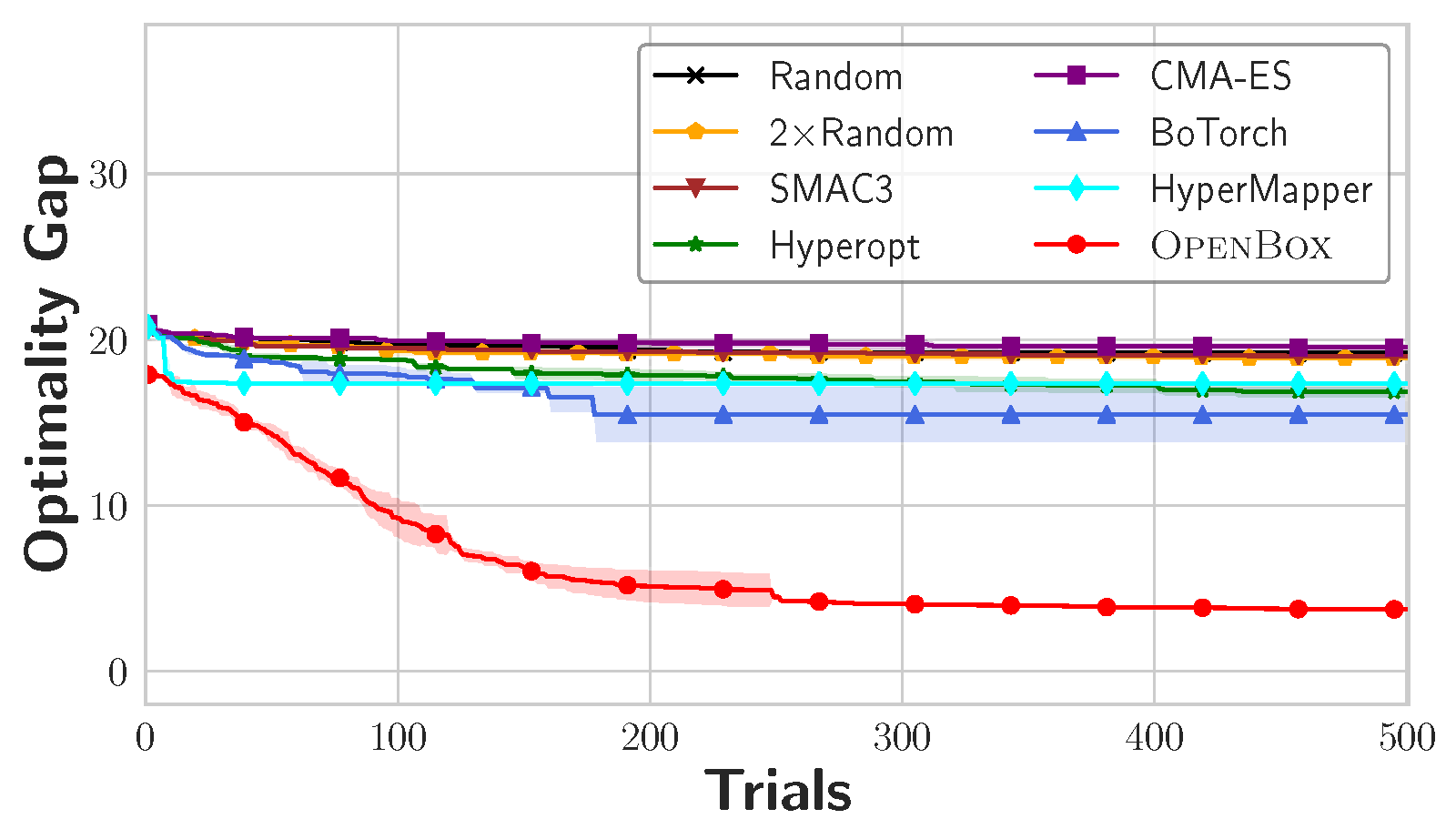
Figure 3. Scalability of the input dimensions on Ackley.

Setup:

Problem: synthetic function Ackley with different input dimensions (4, 8, 16 and 32).
Budget: 300 to 500 iterations depend on the problem difficulty.
Metrics: Optimal gap is the gap between the best found value and the optimal value.
Algorithm in OpenBox: Gaussian Process with Expected Improvement (auto-selected).

To demonstrate the scalability of OpenBox, we conduct experiments on the synthetic function Ackley with different input dimensions. Figure 3 shows the optimal gap of each baseline with the growth of input dimensions. We observe that OpenBox is the only system that achieves consistent and excellent results when the dimensions of the hyperparameter space grow larger. When solving Ackley with 16 and 32-dimensional inputs, OpenBox achieves more than 10× speedups over the other baselines.

Parallel Experiment#

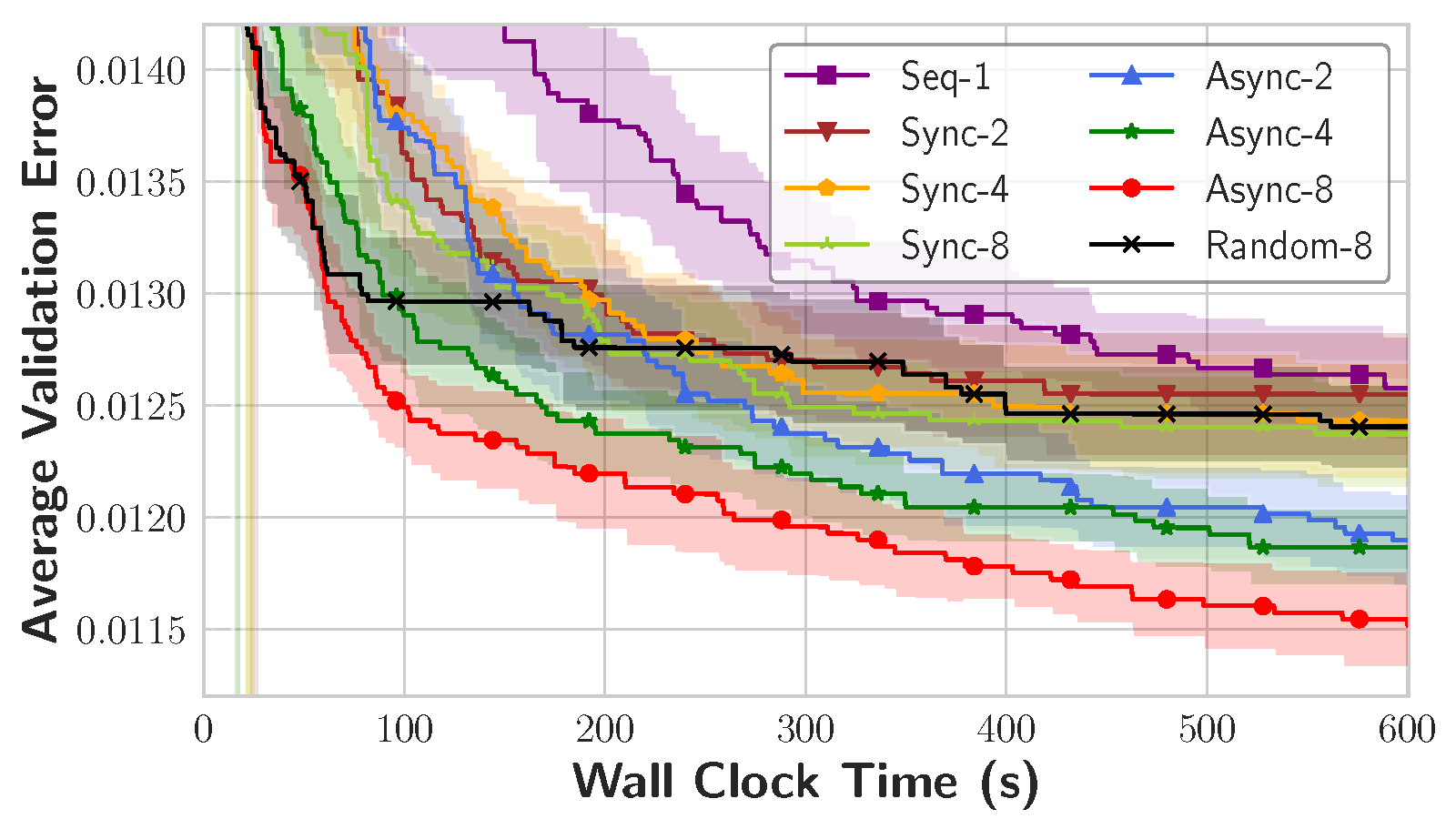
Figure 4: Parallel LightGBM tuning task on optdigits.

Setup:

Problem: tuning LightGBM on optdigits in parallel.
Budget: 600 seconds.
Metrics: Average validation error.
Algorithm in OpenBox: Gaussian Process with Expected Improvement. For parallel tuning, median imputation algorithm is used (auto-selected).

We conduct an experiment to tune the hyper-parameters of LightGBM in parallel on optdigits with a budget of 600 seconds. Figure 4 shows the average validation error with different parallel modes and the number of workers. The asynchronous mode of OpenBox with 8 workers achieves the best results and outperforms Random Search with 8 workers by a wide margin. It brings a speedup of 8× over the sequential mode, which is close to the ideal speedup.

Scalability Experiments on Hyper-parameter Types#



(a) SVM on cpu_act	(b) NAS-Bench-201 CIFAR100

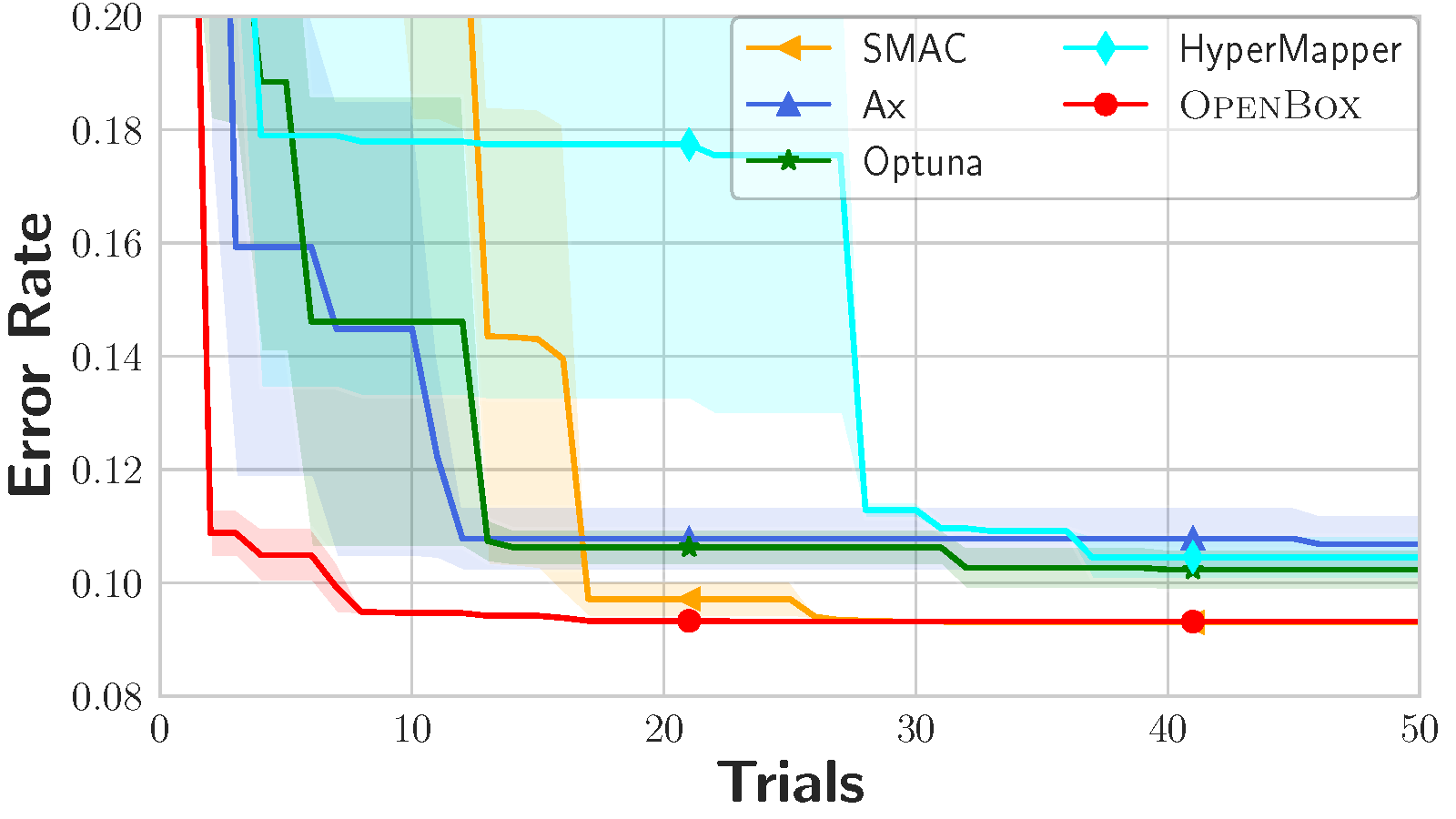
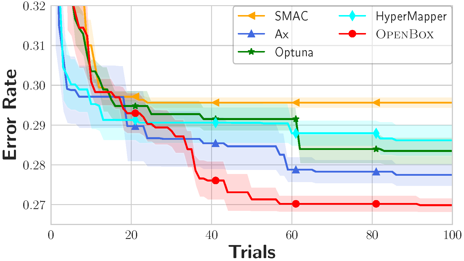
Figure 5: Scalability of hyper-parameter types.

Table 3: The search space of SVM classifier.

Hyper-parameter	Type	Range
penalty	categorical	{l1, l2}
loss	categorical	{hinge, squared_hinge}
dual	categorical	{True, False }
tol	float (log)	[1e-5, 1e-1]
C	float (log)	[2e-5, 2e15]

Table 4: The search space of NAS-Bench-201.

Hyper-parameter	Type	Range
op1	categorical	{none, skip_connect, nor_conv_1x1, nor_conv_3x3, avg_pool_3x3}
op2	categorical	{none, skip_connect, nor_conv_1x1, nor_conv_3x3, avg_pool_3x3}
op3	categorical	{none, skip_connect, nor_conv_1x1, nor_conv_3x3, avg_pool_3x3}
op4	categorical	{none, skip_connect, nor_conv_1x1, nor_conv_3x3, avg_pool_3x3}
op5	categorical	{none, skip_connect, nor_conv_1x1, nor_conv_3x3, avg_pool_3x3}

Setup:

Problems: (1) Tuning SVM classifier on the cpu act dataset (OpenML id 761). 2 floating and 3 categorical hyper-parameters. (2) Neural architecture search benchmark NAS-Bench-201 on CIFAR100 dataset. 5 categorical hyper-parameters.
Budget: 50 or 100 iterations.
Metrics: Error rate.
Algorithm in OpenBox: Probabilistic Random Forest (PRF) with Expected Improvement (auto-selected). The probabilistic random forest is auto-selected as the surrogate model instead of Gaussian process (GP), because there are more categorical hyper-parameters than continuous hyper-parameters in the search space.
Algorithm in other systems: Selected based on their documentation or default choice. Please note that the other components in each system, such as the initial design and acquisition function optimizer, can also affect the results.
- SMAC: random forest with log EI.
- Ax: Gaussian process (gpytorch) with EI.
- Optuna: TPE algorithm.
- HyperMapper: random forest with EI.

Note: We compare Ax instead of BoTorch in this experiment, since Ax extends BoTorch to support categorical hyper-parameters.

To demonstrate the scalability of OpenBox when dealing with different hyper-parameter types, we conduct experiments on two tasks. In the first task, each method tunes an SVM classifier with a mixed-type space of 2 floating and 3 categorical hyper-parameters. In the second task, each method searches the best neural architecture defined by 5 categorical hyper-parameters on CIFAR100 of NAS-Bench-201. As shown in Figure 5, OpenBox outperforms the other baselines, which support categorical hyper-parameters, on both tasks in terms of convergence speed and stability.