Multi-Objective with Constraints
In this tutorial, we will introduce how to optimize constrained multiple objectives problem with OpenBox.
Problem Setup
We use constrained multi-objective problem CONSTR in this example. As CONSTR is a built-in function, its search space and objective function are wrapped as follows:
from openbox.benchmark.objective_functions.synthetic import CONSTR

prob = CONSTR()
dim = 2
initial_runs = 2 * (dim + 1)
import numpy as np
from openbox import space as sp
params = {'x1': (0.1, 10.0),
          'x2': (0.0, 5.0)}
space = sp.Space()
space.add_variables([sp.Real(k, *v) for k, v in params.items()])

def objective_funtion(config: sp.Configuration):
    X = np.array(list(config.get_dictionary().values()))

    result = dict()
    obj1 = X[..., 0]
    obj2 = (1.0 + X[..., 1]) / X[..., 0]
    result['objectives'] = np.stack([obj1, obj2], axis=-1)

    c1 = 6.0 - 9.0 * X[..., 0] - X[..., 1]
    c2 = 1.0 - 9.0 * X[..., 0] + X[..., 1]
    result['constraints'] = np.stack([c1, c2], axis=-1)

    return result
After evaluation, the objective function returns a dict (Recommended).
The result dictionary should contain:
'objectives': A list/tuple of objective values (to be minimized). In this example, we have only one objective so the tuple contains a single value.'constraints': A list/tuple of constraint values. Non-positive constraint values (“<=0”) imply feasibility.
Optimization
from openbox import Optimizer
opt = Optimizer(
    prob.evaluate,
    prob.config_space,
    num_objectives=prob.num_objectives,
    num_constraints=prob.num_constraints,
    max_runs=100,
    surrogate_type='gp',                # try using 'auto'!
    acq_type='ehvic',                   # try using 'auto'!
    acq_optimizer_type='random_scipy',  # try using 'auto'!
    initial_runs=initial_runs,
    init_strategy='sobol',
    ref_point=prob.ref_point,
    task_id='moc',
    random_state=1,
    # Have a try on the new HTML visualization feature!
    # visualization='advanced',   # or 'basic'. For 'advanced', run 'pip install "openbox[extra]"' first
    # auto_open_html=True,        # open the visualization page in your browser automatically
)
history = opt.run()
Here we create a Optimizer instance, and pass the objective function
and the search space to it.
The other parameters are:
num_objectivesandnum_constraintsset how many objectives and constraints the objective function will return. In this example,num_objectives=2andnum_constraints=2.max_runs=100means the optimization will take 100 rounds (optimizing the objective function 100 times).surrogate_type='gp'. For mathematical problem, we suggest using Gaussian Process ('gp') as Bayesian surrogate model. For practical problems such as hyperparameter optimization (HPO), we suggest using Random Forest ('prf'). Set to'auto'to enable automatic algorithm selection.acq_type='ehvic'. Use EHVIC(Expected Hypervolume Improvement with Constraint) as Bayesian acquisition function. Set to'auto'to enable automatic algorithm selection.acq_optimizer_type='random_scipy'. For mathematical problems, we suggest using'random_scipy'as acquisition function optimizer. For practical problems such as hyperparameter optimization (HPO), we suggest using'local_random'. Set to'auto'to enable automatic algorithm selection.initial_runssets how many configurations are suggested byinit_strategybefore the optimization loop.init_strategy='sobol'sets the strategy to suggest the initial configurations.ref_pointspecifies the reference point, which is the upper bound on the objectives used for computing hypervolume. If using EHVI method, a reference point must be provided. In practice, the reference point can be set 1) using domain knowledge to be slightly worse than the upper bound of objective values, where the upper bound is the maximum acceptable value of interest for each objective, or 2) using a dynamic reference point selection strategy.task_idis set to identify the optimization process.visualization:'none','basic'or'advanced'. See HTML Visualization.auto_open_html: whether to open the visualization page in your browser automatically. See HTML Visualization.
Then, opt.run() is called to start the optimization process.
Visualization
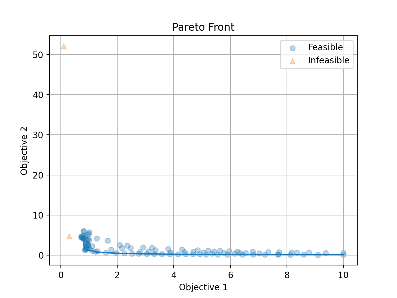
Since we optimize both objectives at the same time, we get a pareto front as the result.
Call opt.get_history().plot_pareto_front() to plot the pareto front.
Please note that plot_pareto_front only works when the number of objectives is 2 or 3.
import matplotlib.pyplot as plt

history = opt.get_history()
# plot pareto front
if history.num_objectives in [2, 3]:
    history.plot_pareto_front()  # support 2 or 3 objectives
    plt.show()
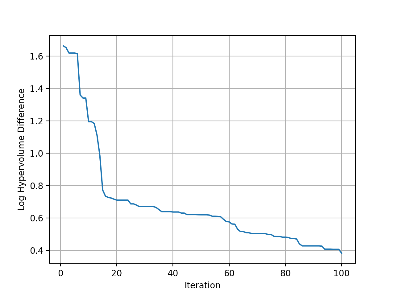
Then plot the hypervolume difference during the optimization compared to the ideal pareto front.
# plot hypervolume (optimal hypervolume of CONSTR is approximated using NSGA-II)
history.plot_hypervolumes(optimal_hypervolume=92.02004226679216, logy=True)
plt.show()
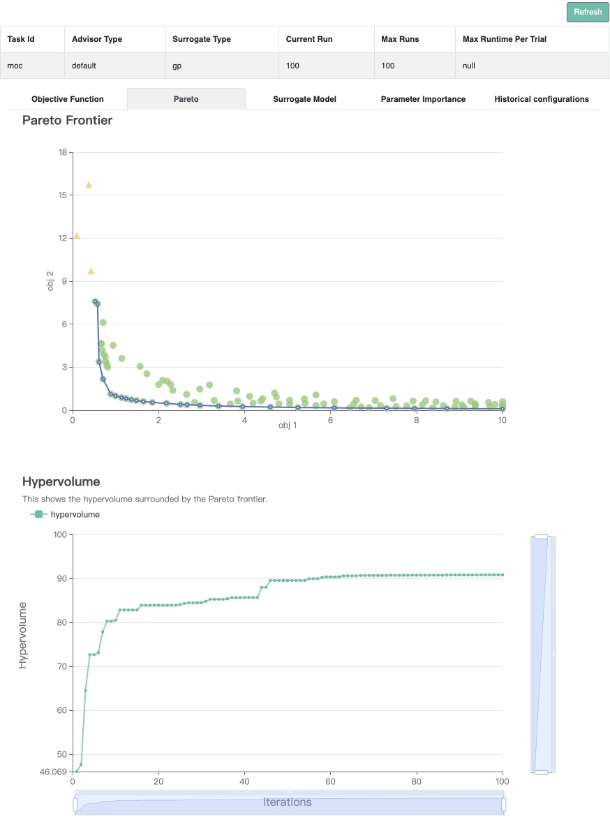
(New Feature!)
Call history.visualize_html() to visualize the optimization process in an HTML page.
For show_importance and verify_surrogate, run pip install "openbox[extra]" first.
See HTML Visualization for more details.
history.visualize_html(open_html=True, show_importance=True,
                       verify_surrogate=True, optimizer=opt)