Quick Start
This tutorial helps you run your first example with OpenBox.
Space Definition
First, define a search space.
from openbox import space as sp

# Define Search Space
space = sp.Space()
x1 = sp.Real("x1", -5, 10, default_value=0)
x2 = sp.Real("x2", 0, 15, default_value=0)
space.add_variables([x1, x2])
In this example, we create an empty search space, and then add two real (floating-point) variables into it.
The first variable x1 ranges from -5 to 10, and the second one x2 ranges from 0 to 15.
OpenBox also supports other types of variables.
Here are examples of how to define Int and Categorical variables:
from openbox import space as sp

i = sp.Int("i", 0, 100)
kernel = sp.Categorical("kernel", ["rbf", "poly", "sigmoid"], default_value="rbf")
For advanced usage, please refer to Problem Definition with Complex Search Space.
The space in OpenBox is implemented based on ConfigSpace package. For more usage, also refer to ConfigSpace’s documentation.
Objective Definition
Second, define the objective function to be optimized. Note that OpenBox aims to minimize the objective function. Here we provide an example of the Branin function.
import numpy as np

# Define Objective Function
def branin(config):
    x1, x2 = config['x1'], config['x2']
    y = (x2-5.1/(4*np.pi**2)*x1**2+5/np.pi*x1-6)**2+10*(1-1/(8*np.pi))*np.cos(x1)+10
    return {'objectives': [y]}
The objective function takes as input a configuration sampled from space
and outputs the objective value.
Optimization
After defining the search space and the objective function, we can run the optimization process as follows:
from openbox import Optimizer

# Run
opt = Optimizer(
    branin,
    space,
    max_runs=50,
    surrogate_type='gp',          # try using 'auto'!
    task_id='quick_start',
    # Have a try on the new HTML visualization feature!
    # visualization='advanced',   # or 'basic'. For 'advanced', run 'pip install "openbox[extra]"' first
    # auto_open_html=True,        # open the visualization page in your browser automatically
)
history = opt.run()
Here we create a Optimizer instance, and pass the objective function branin and the
search space space to it. The other parameters are:
num_objectives=1andnum_constraints=0indicates our branin function returns a single value with no constraint.max_runs=50means the optimization will take 50 rounds (optimizing the objective function 50 times).surrogate_type='gp'. For mathematical problems, we suggest using Gaussian Process ('gp') as Bayesian surrogate model. For practical problems such as hyperparameter optimization (HPO), we suggest using Random Forest ('prf'). Set to'auto'to enable automatic algorithm selection.task_idis set to identify the optimization process.visualization:'none','basic'or'advanced'. See HTML Visualization.auto_open_html: whether to open the visualization page in your browser automatically. See HTML Visualization.
Then, opt.run() is called to start the optimization process.
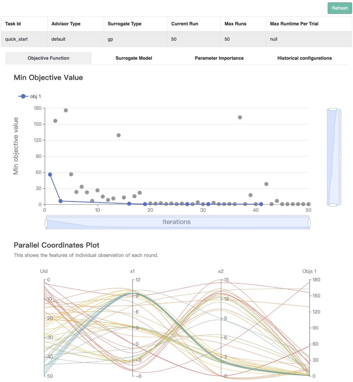
Visualization
After the optimization, opt.run() returns the optimization history.
Call print(history) to see the result:
print(history)
+-------------------------+-------------------+
| Parameters              | Optimal Value     |
+-------------------------+-------------------+
| x1                      | -3.138277         |
| x2                      | 12.254526         |
+-------------------------+-------------------+
| Optimal Objective Value | 0.398096578033325 |
+-------------------------+-------------------+
| Num Configs             | 50                |
+-------------------------+-------------------+
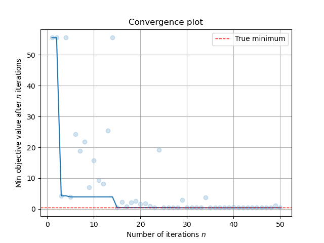
Call history.plot_convergence() to visualize the optimization process:
import matplotlib.pyplot as plt
history.plot_convergence(true_minimum=0.397887)
plt.show()
Call print(history.get_importance()) to print the parameter importance:
(Note that you need to install the pyrfr package to use this function.
Pyrfr Installation Guide
print(history.get_importance())
+------------+------------+
| Parameters | Importance |
+------------+------------+
| x1         | 0.488244   |
| x2         | 0.327570   |
+------------+------------+
(New Feature!)
Call history.visualize_html() to visualize the optimization process in an HTML page.
For show_importance and verify_surrogate, run pip install "openbox[extra]" first.
See HTML Visualization for more details.
history.visualize_html(open_html=True, show_importance=True,
                       verify_surrogate=True, optimizer=opt)