Single-Objective with Constraints¶

In this tutorial, we will introduce how to optimize a constrained problem with OpenBox.

Problem Setup¶

First, define search space and define objective function to minimize. Here we use the constrained Mishra function.

import numpy as np
from openbox import space as sp

def mishra(config: sp.Configuration):
    X = np.array([config['x%d' % i] for i in range(2)])
    x, y = X[0], X[1]
    t1 = np.sin(y) * np.exp((1 - np.cos(x))**2)
    t2 = np.cos(x) * np.exp((1 - np.sin(y))**2)
    t3 = (x - y)**2

    result = dict()
    result['objectives'] = [t1 + t2 + t3, ]
    result['constraints'] = [np.sum((X + 5)**2) - 25, ]
    return result

params = {
    'float': {
        'x0': (-10, 0, -5),
        'x1': (-6.5, 0, -3.25)
    }
}
space = sp.Space()
space.add_variables([
    sp.Real(name, *para) for name, para in params['float'].items()
])

After evaluation, the objective function returns a dict (Recommended). The result dictionary should contain:

'objectives': A list/tuple of objective values (to be minimized). In this example, we have only one objective so the tuple contains a single value.
'constraints': A list/tuple of constraint values. Non-positive constraint values (“<=0”) imply feasibility.

Optimization¶

After defining the search space and the objective function, we can run the optimization process as follows:

from openbox import Optimizer

opt = Optimizer(
    mishra,
    space,
    num_constraints=1,
    num_objectives=1,
    surrogate_type='gp',                # try using 'auto'!
    acq_optimizer_type='random_scipy',  # try using 'auto'!
    max_runs=50,
    task_id='soc',
    # Have a try on the new HTML visualization feature!
    # visualization='advanced',   # or 'basic'. For 'advanced', run 'pip install "openbox[extra]"' first
    # auto_open_html=True,        # open the visualization page in your browser automatically
)
history = opt.run()

Here we create a Optimizer instance, and pass the objective function and the search space to it. The other parameters are:

num_objectives=1 and num_constraints=1 indicate that our function returns a single value with one constraint.
max_runs=50 means the optimization will take 50 rounds (optimizing the objective function 50 times).
task_id is set to identify the optimization process.
visualization: 'none', 'basic' or 'advanced'. See HTML Visualization.
auto_open_html: whether to open the visualization page in your browser automatically. See HTML Visualization.

Then, opt.run() is called to start the optimization process.

Visualization¶

After the optimization, opt.run() returns the optimization history. Or you can call opt.get_history() to get the history. Then, call print(history) to see the result:

history = opt.get_history()
print(history)

+-------------------------+---------------------+
| Parameters              | Optimal Value       |
+-------------------------+---------------------+
| x0                      | -3.172421           |
| x1                      | -1.506397           |
+-------------------------+---------------------+
| Optimal Objective Value | -105.72769850551406 |
+-------------------------+---------------------+
| Num Configs             | 50                  |
+-------------------------+---------------------+

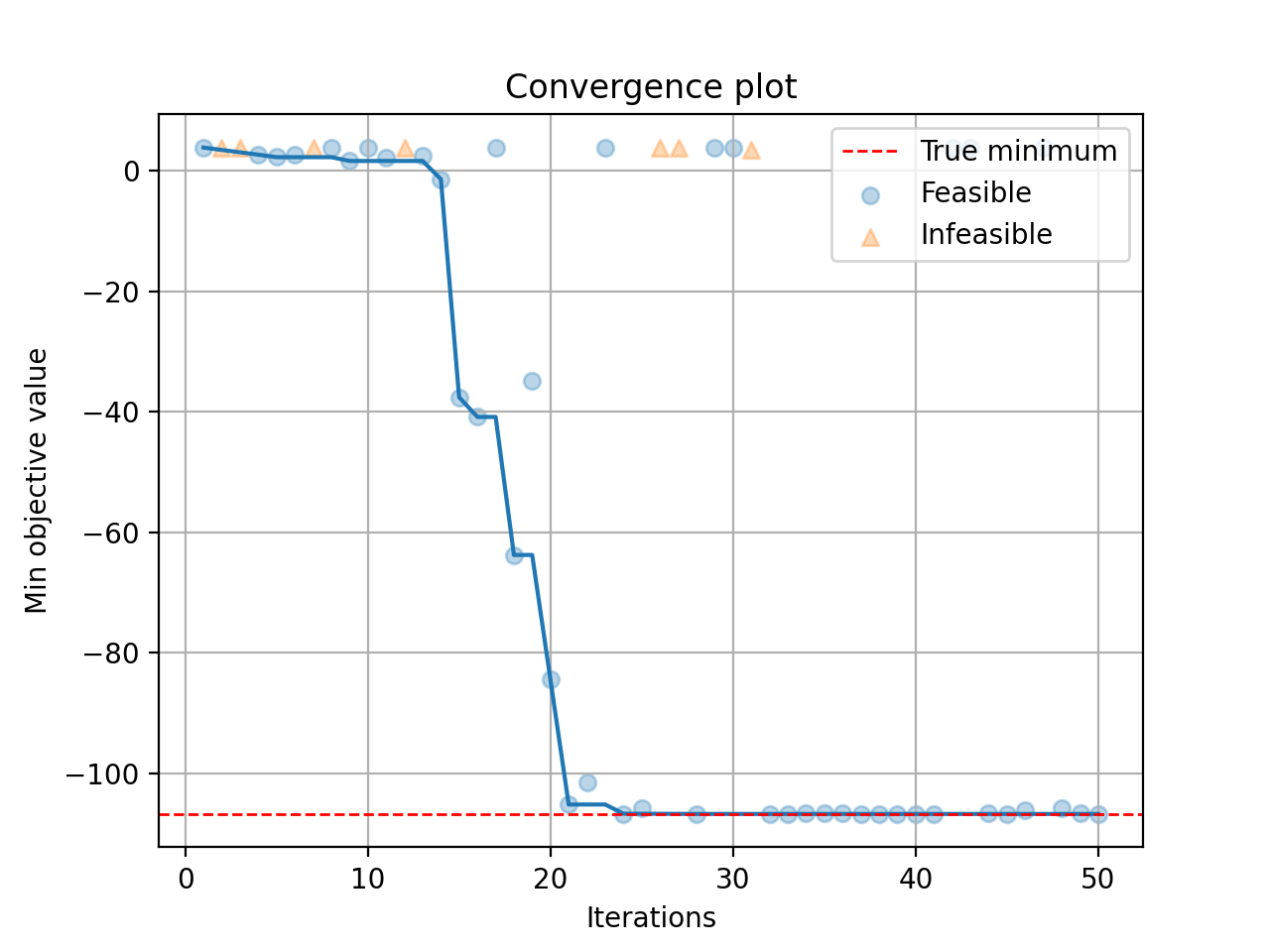
Call history.plot_convergence() to visualize the optimization process:

import matplotlib.pyplot as plt
history.plot_convergence(true_minimum=-106.7645367)
plt.show()

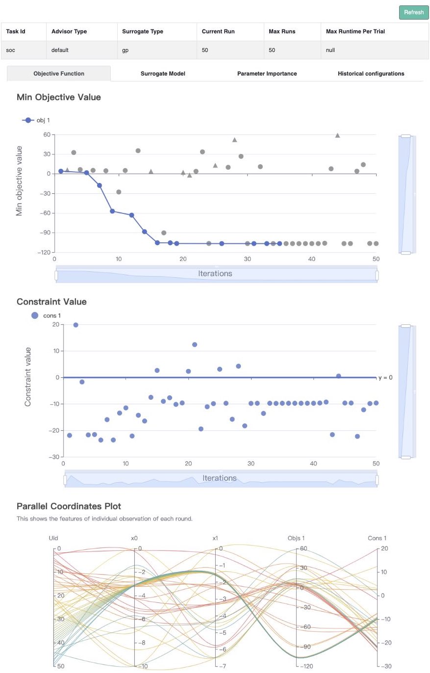
(New Feature!) Call history.visualize_html() to visualize the optimization process in an HTML page. For show_importance and verify_surrogate, run pip install "openbox[extra]" first. See HTML Visualization for more details.

history.visualize_html(open_html=True, show_importance=True,
                       verify_surrogate=True, optimizer=opt)