单目标的黑盒优化#
本教程介绍如何使用OpenBox为机器学习任务调优超参数。
数据准备#
首先,给机器学习模型 准备数据。 这里我们用sklearn中的digits数据集。
# prepare your data
from sklearn.model_selection import train_test_split
from sklearn.datasets import load_digits

X, y = load_digits(return_X_y=True)
x_train, x_test, y_train, y_test = train_test_split(X, y, test_size=0.2, stratify=y, random_state=1)
问题设置#
其次,定义搜索空间和想要最小化的目标函数。 这里,我们使用 LightGBM – 一个由微软开发的梯度提升算法框架作为分类模型。
from openbox import space as sp
from sklearn.metrics import balanced_accuracy_score
from lightgbm import LGBMClassifier


def get_configspace():
    space = sp.Space()
    n_estimators = sp.Int("n_estimators", 100, 1000, default_value=500, q=50)
    num_leaves = sp.Int("num_leaves", 31, 2047, default_value=128)
    max_depth = sp.Constant('max_depth', 15)
    learning_rate = sp.Real("learning_rate", 1e-3, 0.3, default_value=0.1, log=True)
    min_child_samples = sp.Int("min_child_samples", 5, 30, default_value=20)
    subsample = sp.Real("subsample", 0.7, 1, default_value=1, q=0.1)
    colsample_bytree = sp.Real("colsample_bytree", 0.7, 1, default_value=1, q=0.1)
    space.add_variables([n_estimators, num_leaves, max_depth, learning_rate, min_child_samples, subsample,
                      colsample_bytree])
    return space


def objective_function(config: sp.Configuration):
    params = config.get_dictionary().copy()
    params['n_jobs'] = 2
    params['random_state'] = 47

    model = LGBMClassifier(**params)
    model.fit(x_train, y_train)
    y_pred = model.predict(x_test)

    loss = 1 - balanced_accuracy_score(y_test, y_pred)  # minimize
    return dict(objectives=[loss])
下面给出了一些定义搜索空间的提示:
当我们定义
n_estimators时,我们设置q=50, 表示超参数配置采样的间隔是50。当我们定义
learning_rate时,我们设置log=True, 表示超参数的值以对数方式采样。
objective_function 的输入是一个从 space 中采样的 Configuration 实例。
你可以调用 config.get_dictionary().copy() 来把 Configuration 转化成一个 Python dict。
在这个超参数优化任务中,一旦采样出一个新的超参数配置,我们就根据输入配置构建模型。 然后,对模型进行拟合,评价模型的预测性能。 这些步骤在目标函数中执行。
评估性能后,目标函数需要返回一个 dict (推荐)
其中的结果包含:
'objectives':一个 要被最小化目标值 的 列表/元组。 在这个例子中,我们只有一个目标,所以这个元组只包含一个值。'constraints':一个含有 约束值 的 列表/元组。 如果问题没有约束,返回None或者不要把这个 key 放入字典。 非正的约束值 (“<=0”) 表示可行。
除了返回字典以外,对于无约束条件的单目标优化问题,我们也可以返回一个单独的值。
优化#
在定义了搜索空间和目标函数后,我们按如下方式运行优化过程:
from openbox import Optimizer

# Run
opt = Optimizer(
    objective_function,
    get_configspace(),
    num_objectives=1,
    num_constraints=0,
    max_runs=100,
    surrogate_type='prf',
    task_id='so_hpo',
    # Have a try on the new HTML visualization feature!
    # visualization='advanced',   # or 'basic'. For 'advanced', run 'pip install "openbox[extra]"' first
    # auto_open_html=True,        # open the visualization page in your browser automatically
)
history = opt.run()
这里我们创建一个 Optimizer 实例,传入目标函数和配置空间。
其它的参数是:
num_objectives=1和num_constraints=0表示我们的函数返回一个没有约束的单目标值。max_runs=100表示优化会进行100轮(优化目标函数100次)。surrogate_type='prf'对于数学问题,我们推荐用高斯过程 ('gp') 做贝叶斯优化的替代模型。 对于实际问题,比如超参数优化(HPO)问题,我们推荐使用随机森林('prf')。task_id用来识别优化过程。visualization:'none','basic'或'advanced'。 详见 可视化网页。auto_open_html: 是否自动在浏览器中打开可视化网页。 详见 可视化网页。
然后,调用 opt.run() 启动优化过程。
可视化#
在优化完成后,opt.run() 会返回优化的历史过程。或者你可以调用 opt.get_history() 来获得优化历史。
接下来,调用 print(history) 来查看结果:
history = opt.get_history()
print(history)
+-------------------------+----------------------+
| Parameters              | Optimal Value        |
+-------------------------+----------------------+
| colsample_bytree        | 0.800000             |
| learning_rate           | 0.018402             |
| max_depth               | 15                   |
| min_child_samples       | 15                   |
| n_estimators            | 200                  |
| num_leaves              | 723                  |
| subsample               | 0.800000             |
+-------------------------+----------------------+
| Optimal Objective Value | 0.022305877305877297 |
+-------------------------+----------------------+
| Num Configs             | 100                  |
+-------------------------+----------------------+
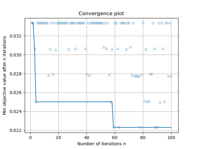
调用 history.plot_convergence() 来可视化优化过程:
import matplotlib.pyplot as plt
history.plot_convergence()
plt.show()
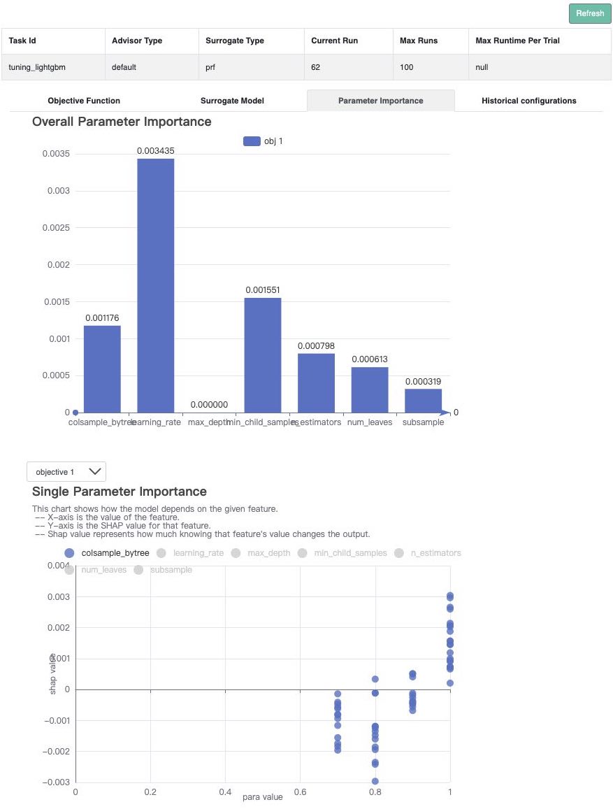
调用 print(history.get_importance()) 来输出超参数的重要性:
(注意:使用该功能需要额外安装pyrfr包:Pyrfr安装教程
print(history.get_importance())
+-------------------+------------+
| Parameters        | Importance |
+-------------------+------------+
| learning_rate     | 0.293457   |
| min_child_samples | 0.101243   |
| n_estimators      | 0.076895   |
| num_leaves        | 0.069107   |
| colsample_bytree  | 0.051856   |
| subsample         | 0.010067   |
| max_depth         | 0.000000   |
+-------------------+------------+
在本任务中,3个最重要的超参数是 learning_rate,min_child_samples,和 n_estimators。
(新功能!)
调用 history.visualize_html() 来显示可视化网页。
对于 show_importance 和 verify_surrogate,需要先运行 pip install "openbox[extra]"。
详细说明请参考 可视化网页。
history.visualize_html(open_html=True, show_importance=True,
                       verify_surrogate=True, optimizer=opt)