多目标黑盒优化
本教程介绍如何使用OpenBox解决多目标优化问题。
问题设置
在这个例子中,我们使用了具有三个输入维度的的多目标问题ZDT2。OpenBox内置了ZDT2函数,其搜索空间和目标函数被包装如下:
from openbox.benchmark.objective_functions.synthetic import ZDT2

dim = 3
prob = ZDT2(dim=dim)
import numpy as np
from openbox import space as sp
params = {'x%d' % i: (0, 1) for i in range(1, dim+1)}
space = sp.Space()
space.add_variables([sp.Real(k, *v) for k, v in params.items()])

def objective_function(config: sp.Configuration):
    X = np.array(list(config.get_dictionary().values()))
    f_0 = X[..., 0]
    g = 1 + 9 * X[..., 1:].mean(axis=-1)
    f_1 = g * (1 - (f_0 / g)**2)

    result = dict()
    result['objectives'] = np.stack([f_0, f_1], axis=-1)
    return result
在评估后,目标函数需要返回一个 dict (推荐)
其中的结果包含:
'objectives':一个 要被最小化目标值 的 列表/元组。 在这个例子中,我们只有一个目标,所以这个元组只包含一个值。'constraints':一个含有 约束值 的 列表/元组。 如果问题没有约束,返回None或者不要把这个 key 放入字典。 非正的约束值 (“<=0”) 表示可行。
优化
from openbox import Optimizer
opt = Optimizer(
    prob.evaluate,
    prob.config_space,
    num_objectives=prob.num_objectives,
    num_constraints=0,
    max_runs=50,
    surrogate_type='gp',                # try using 'auto'!
    acq_type='ehvi',                    # try using 'auto'!
    acq_optimizer_type='random_scipy',  # try using 'auto'!
    initial_runs=2*(dim+1),
    init_strategy='sobol',
    ref_point=prob.ref_point,
    task_id='mo',
    random_state=1,
    # Have a try on the new HTML visualization feature!
    # visualization='advanced',   # or 'basic'. For 'advanced', run 'pip install "openbox[extra]"' first
    # auto_open_html=True,        # open the visualization page in your browser automatically
)
opt.run()
这里我们创建一个 Optimizer 实例,并传入目标函数和搜索空间。
其它的参数是:
num_objectives和num_constraints设置目标函数将返回多少目标和约束。在这个例子中,num_objectives=2。max_runs=50表示优化会进行50轮(优化目标函数50次)。surrogate_type='gp'对于数学问题,我们推荐用高斯过程 ('gp') 做贝叶斯优化的替代模型。 对于实际问题,比如超参数优化(HPO)问题,我们推荐使用随机森林('prf')。 设置为'auto'来启用自动化算法选择。acq_type='ehvi'用 EHVI(Expected Hypervolume Improvement) 作为贝叶斯优化的acquisition function。 对于超过三个目标的问题,请使用MESMO('mesmo') 或 USEMO('usemo')。 设置为'auto'来启用自动化算法选择。acq_optimizer_type='random_scipy'. 对于数学问题,我们推荐用'random_scipy'作为 acquisition function 的优化器。 对于实际问题,比如超参数优化(HPO)问题,我们推荐使用'local_random'。 设置为'auto'来启用自动化算法选择。initial_runs设置在优化循环之前,init_strategy推荐使用的配置数量。init_strategy='sobol'设置建议初始配置的策略。ref_point指定参考点,它是用于计算超体积的目标的上限。 如果使用EHVI方法,则必须提供参考点。 在实践中,可以1)使用领域知识将参考点设置为略差于目标值的上界,其中上界是每个目标感兴趣的最大可接受值,或者2)使用动态的参考点选择策略。task_id用来识别优化过程。visualization:'none','basic'或'advanced'。 详见 可视化网页。auto_open_html: 是否自动在浏览器中打开可视化网页。 详见 可视化网页。
然后,调用 opt.run() 启动优化过程。
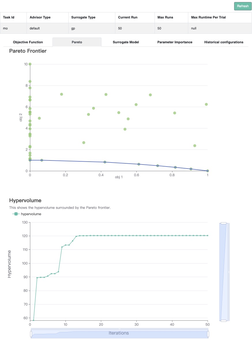
可视化
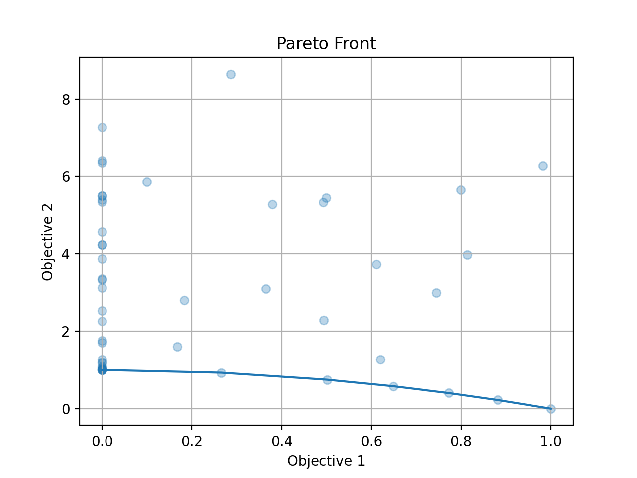
由于我们同时优化了这两个目标,我们得到了一个帕累托前沿(pareto front)作为结果。
调用 opt.get_history().plot_pareto_front() 来绘制帕累托前沿。
请注意,plot_pareto_front只在目标数为2或3时可用。
import matplotlib.pyplot as plt

history = opt.get_history()
# plot pareto front
if history.num_objectives in [2, 3]:
    history.plot_pareto_front()  # support 2 or 3 objectives
    plt.show()
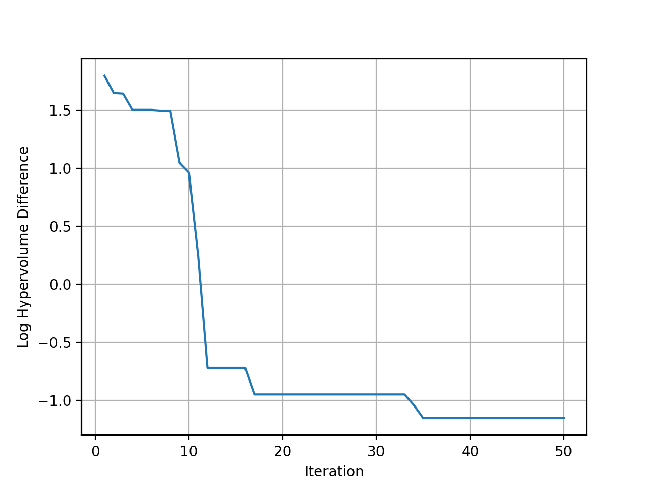
然后绘制优化过程中与理想帕累托前沿相比的hypervolume差。
# plot hypervolume
history.plot_hypervolumes(optimal_hypervolume=prob.max_hv, logy=True)
plt.show()
(新功能!)
调用 history.visualize_html() 来显示可视化网页。
对于 show_importance 和 verify_surrogate,需要先运行 pip install "openbox[extra]"。
详细说明请参考 可视化网页。
history.visualize_html(open_html=True, show_importance=True,
                       verify_surrogate=True, optimizer=opt)