# OpenBox: A Generalized Black-box Optimization Service (1)
 ## Introduction
Recent years have witnessed the rapid development of artificial intelligence and machine learning. Machine learning models have been widely applied to solve practical problems, such as data prediction and analysis, face recognition, product recommendation, etc. However, the application of machine learning is not easy, as the choice of hyperparameter configurations has a great impact on the model performance. Hyperparameter optimization, which is a typical example of black-box optimization, has become one of the important challenges of machine learning. There is no analytical form or gradient information of the optimization objective, and the evaluation is expensive. Its goal is to find the global optimum within a limited budget of evaluation times.
OpenBox is an open-source system designed for black-box optimization. Based on Bayesian optimization, OpenBox can solve black-box optimization problems efficiently. It supports not only traditional single objective black-box optimization problems (e.g., hyperparameter optimization), but also multi-objective optimization, optimization with constraints, multiple parameter types, transfer learning, distributed parallel evaluation, multi-fidelity optimization, etc. Moreover, OpenBox provides both standalone local usage and online optimization service. Users can monitor and manage the optimization tasks on web pages, and also deploy their private optimization service.
In this article, we will first introduce black-box optimization, and then OpenBox -- our generalized open source black-box optimization service.
## What is Black-box Optimization?
In white-box optimization, the specific form of the problem is known. For example, we can solve linear regression by analytic formula, or we can optimize deep neural networks by their gradient information. However, in black-box optimization, the objective function has no analytical form so that information such as the derivative of the objective function is unavailable. We cannot use the characteristics of the optimization objective to obtain its global optimum.
## Introduction
Recent years have witnessed the rapid development of artificial intelligence and machine learning. Machine learning models have been widely applied to solve practical problems, such as data prediction and analysis, face recognition, product recommendation, etc. However, the application of machine learning is not easy, as the choice of hyperparameter configurations has a great impact on the model performance. Hyperparameter optimization, which is a typical example of black-box optimization, has become one of the important challenges of machine learning. There is no analytical form or gradient information of the optimization objective, and the evaluation is expensive. Its goal is to find the global optimum within a limited budget of evaluation times.
OpenBox is an open-source system designed for black-box optimization. Based on Bayesian optimization, OpenBox can solve black-box optimization problems efficiently. It supports not only traditional single objective black-box optimization problems (e.g., hyperparameter optimization), but also multi-objective optimization, optimization with constraints, multiple parameter types, transfer learning, distributed parallel evaluation, multi-fidelity optimization, etc. Moreover, OpenBox provides both standalone local usage and online optimization service. Users can monitor and manage the optimization tasks on web pages, and also deploy their private optimization service.
In this article, we will first introduce black-box optimization, and then OpenBox -- our generalized open source black-box optimization service.
## What is Black-box Optimization?
In white-box optimization, the specific form of the problem is known. For example, we can solve linear regression by analytic formula, or we can optimize deep neural networks by their gradient information. However, in black-box optimization, the objective function has no analytical form so that information such as the derivative of the objective function is unavailable. We cannot use the characteristics of the optimization objective to obtain its global optimum.
 The figure above is a schematic diagram of a black-box function. The black-box function can be viewed in terms of its inputs and outputs, without any knowledge of its internal workings. We can only continuously input data into the black-box function, and then use the outputs to guess the structure information.
Taking hyperparameter optimization of machine learning as an example, our goal is to find a hyperparameter configuration that makes the machine learning model perform best. Therefore, the input of the black-box function is a hyperparameter configuration of the model, and the output is the performance evaluation of the model by training the model using this hyperparameter configuration and making predictions. The relationship between the model performance and the hyperparameters can not be described by specific expressions.
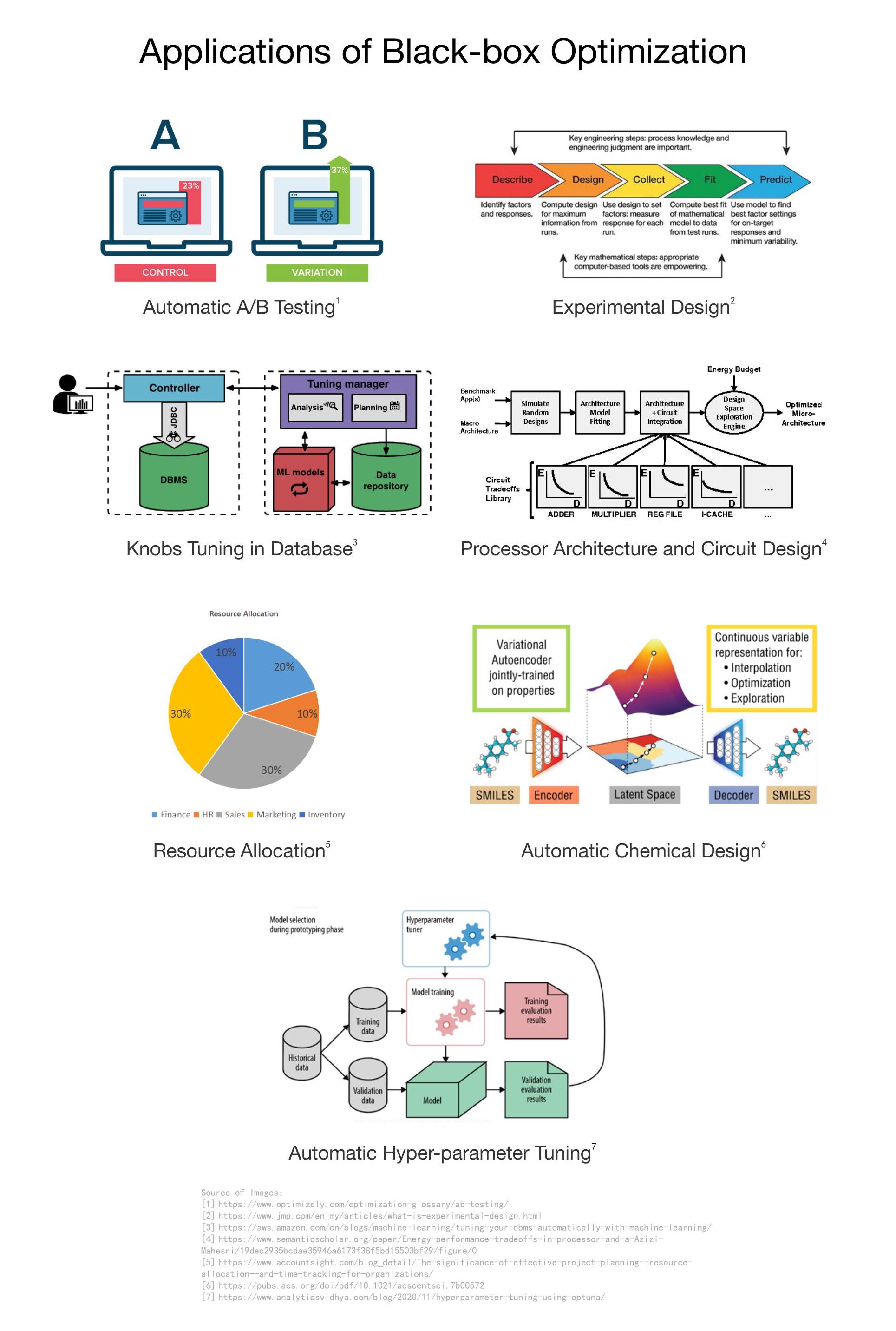
In addition to automatic hyperparameter tuning, black-box optimization has a wide range of applications in many fields, such as automatic A/B testing, experimental design, knobs tuning in database, processor architecture and circuit design, resource allocation, automatic chemical design, etc. (as shown in the figure below).
The figure above is a schematic diagram of a black-box function. The black-box function can be viewed in terms of its inputs and outputs, without any knowledge of its internal workings. We can only continuously input data into the black-box function, and then use the outputs to guess the structure information.
Taking hyperparameter optimization of machine learning as an example, our goal is to find a hyperparameter configuration that makes the machine learning model perform best. Therefore, the input of the black-box function is a hyperparameter configuration of the model, and the output is the performance evaluation of the model by training the model using this hyperparameter configuration and making predictions. The relationship between the model performance and the hyperparameters can not be described by specific expressions.
In addition to automatic hyperparameter tuning, black-box optimization has a wide range of applications in many fields, such as automatic A/B testing, experimental design, knobs tuning in database, processor architecture and circuit design, resource allocation, automatic chemical design, etc. (as shown in the figure below).
 ### Grid Search & Random Search
Grid search and random search are two naive methods to solve the black-box optimization problem. Grid search is also known as full factorial design. The user specifies a finite set of values for each hyperparameter, and grid search evaluates the Cartesian product of these sets. Obviously, grid search suffers from the curse of dimensionality, that is, with the increase of the number of hyperparameters, the number of evaluation times required increases exponentially.
Compared with grid search, random search is a more effective method. It will continuously sample hyperparameter randomly and evaluate it within a given resource (e.g., time) constraint. If there are unimportant hyperparameters, when performing grid search, we fix the value of important hyperparameters and try different values of unimportant hyperparameters, resulting in a small difference of evaluation results and low efficiency. However, random search avoids this problem and can search more different objective values corresponding to different important hyperparameters. The figure below shows the difference between grid search and random search.
### Grid Search & Random Search
Grid search and random search are two naive methods to solve the black-box optimization problem. Grid search is also known as full factorial design. The user specifies a finite set of values for each hyperparameter, and grid search evaluates the Cartesian product of these sets. Obviously, grid search suffers from the curse of dimensionality, that is, with the increase of the number of hyperparameters, the number of evaluation times required increases exponentially.
Compared with grid search, random search is a more effective method. It will continuously sample hyperparameter randomly and evaluate it within a given resource (e.g., time) constraint. If there are unimportant hyperparameters, when performing grid search, we fix the value of important hyperparameters and try different values of unimportant hyperparameters, resulting in a small difference of evaluation results and low efficiency. However, random search avoids this problem and can search more different objective values corresponding to different important hyperparameters. The figure below shows the difference between grid search and random search.

Grid Search & Random Search
### Bayesian Optimization
Bayesian optimization is a state-of-the-art black-box optimization framework. For expensive black-box functions, it can find the global minimum within fewer evaluation steps. The probabilistic surrogate model and acquisition function are two key components of Bayesian optimization. The main steps of optimization are as follows:
+ Train surrogate model with historical observations of black-box function.
+ Optimize the acquisition function to get the most promising candidate point to evaluate.
+ Input the chosen point into the black-box function and update observation to the history.
+ Repeat the above steps until a certain budget is exhausted or the expected objective value is achieved.
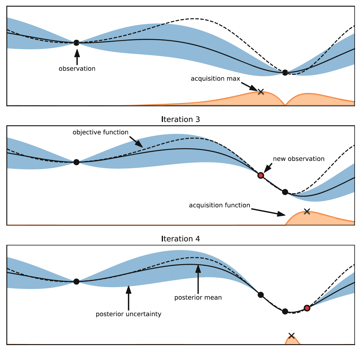 The above figure is an example of Bayesian Optimization in one-dimensional input space. The three diagrams from top to bottom display the sequential optimization process. The black dotted line in the figure represents the real black-box function. In the initial case, two historical observations are used to train the probabilistic surrogate model. The predicted mean is represented by the black solid line, and the predicted variance (i.e. uncertainty) is represented by the blue area. The commonly used surrogate models are Gaussian Process, Random Forest, Tree-structured Parzen Estimator (TPE), etc.
According to the surrogate model, the acquisition function (orange curve in the figure) suggests the most promising candidate input parameters. The acquisition function needs to balance exploration and exploitation, that is, to choose the candidate with higher uncertainty or better predictive performance. Compared with the real black-box function, the evaluation cost of the acquisition function is much lower, so it can be fully optimized. Common acquisition functions include Expected Improvement, Lower Confidence Bound, Probability of Improvement, etc.
After optimizing the acquisition function, we get the candidate input point with the highest acquisition value (X on the orange curve). Then we evaluate this input point on the black-box function and get a new observation. We retrain the surrogate model for the next round of optimization.
## What is OpenBox?
OpenBox is an efficient generalized open-source system for black-box optimization. Its design satisfies the following desiderata:
+ Ease of use: Minimal user effort, and user-friendly visualization for tracking and managing BBO tasks.
+ Consistent performance: Host state-of-the-art optimization algorithms; choose the proper algorithm automatically.
+ Resource-aware management: Give cost-model-based advice to users, e.g., minimal workers or time-budget.
+ Scalability: Scale to dimensions on the number of input variables, objectives, tasks, trials, and parallel evaluations.
+ High efficiency: Effective use of parallel resources, system optimization with transfer-learning and multi-fidelities, etc.
+ Fault tolerance, extensibility, and data privacy protection.
OpenBox is coded with Python. You can visit our project here: .
### Abundant Functionalities
Compared with the existing black-box optimization (hyperparameter optimization) systems, OpenBox supports a wider range of functionality scope, including multi-objective optimization, optimization with constraints, multiple parameter types, transfer learning, distributed parallel evaluation, multi-fidelity optimization, and etc. The supported scenarios of OpenBox and existing systems are compared as follows:
The above figure is an example of Bayesian Optimization in one-dimensional input space. The three diagrams from top to bottom display the sequential optimization process. The black dotted line in the figure represents the real black-box function. In the initial case, two historical observations are used to train the probabilistic surrogate model. The predicted mean is represented by the black solid line, and the predicted variance (i.e. uncertainty) is represented by the blue area. The commonly used surrogate models are Gaussian Process, Random Forest, Tree-structured Parzen Estimator (TPE), etc.
According to the surrogate model, the acquisition function (orange curve in the figure) suggests the most promising candidate input parameters. The acquisition function needs to balance exploration and exploitation, that is, to choose the candidate with higher uncertainty or better predictive performance. Compared with the real black-box function, the evaluation cost of the acquisition function is much lower, so it can be fully optimized. Common acquisition functions include Expected Improvement, Lower Confidence Bound, Probability of Improvement, etc.
After optimizing the acquisition function, we get the candidate input point with the highest acquisition value (X on the orange curve). Then we evaluate this input point on the black-box function and get a new observation. We retrain the surrogate model for the next round of optimization.
## What is OpenBox?
OpenBox is an efficient generalized open-source system for black-box optimization. Its design satisfies the following desiderata:
+ Ease of use: Minimal user effort, and user-friendly visualization for tracking and managing BBO tasks.
+ Consistent performance: Host state-of-the-art optimization algorithms; choose the proper algorithm automatically.
+ Resource-aware management: Give cost-model-based advice to users, e.g., minimal workers or time-budget.
+ Scalability: Scale to dimensions on the number of input variables, objectives, tasks, trials, and parallel evaluations.
+ High efficiency: Effective use of parallel resources, system optimization with transfer-learning and multi-fidelities, etc.
+ Fault tolerance, extensibility, and data privacy protection.
OpenBox is coded with Python. You can visit our project here: .
### Abundant Functionalities
Compared with the existing black-box optimization (hyperparameter optimization) systems, OpenBox supports a wider range of functionality scope, including multi-objective optimization, optimization with constraints, multiple parameter types, transfer learning, distributed parallel evaluation, multi-fidelity optimization, and etc. The supported scenarios of OpenBox and existing systems are compared as follows:
 + Multiple parameter types (FIOC, i.e Float, Integer, Ordinal, and Categorical): input parameters are not limited to float type (real number). For example, the kernel function of Supported Vector Machine is represented by a categorical hyperparameter. Using integer instead of ordinal or categorical type will attach an additional order relationship to parameters, which is not conducive to model optimization.
+ Multi-objective Optimization: Simultaneously optimize multiple different or even conflicting objectives, such as simultaneously optimize the accuracy of the machine learning model and model training/prediction time.
+ Optimization with Constraints: The (black-box) condition should be satisfied while optimizing the objective.
Few existing systems can support the above features at the same time. OpenBox supports not only all the above features but also:
+ Using historical task information to guide the current optimization task, namely transfer learning.
+ Provide parallel optimization algorithm. Support distributed evaluation. Make full use of parallel resources.
+ Multi-fidelity optimization algorithm is provided to further accelerate the search in high evaluation cost scenarios (such as training machine learning models on large datasets).
We will introduce how to use OpenBox in different scenarios in future articles.
### Various Optimization Strategies
OpenBox uses the Bayesian optimization algorithm based on the Random Forest surrogate model by default, which shows outstanding performance on hyperparameter optimization tasks. Compared with the SMAC3 library that uses the same algorithm, OpenBox adopts more optimization strategies, which leads to faster convergence and further improves the performance.
For Bayesian optimization, OpenBox also supports:
+ Gaussian Process surrogate model
+ Tree-structured Parzen Estimator (TPE) model
+ Various acquisition functions, such as EI, PI, LCB, EIC, EHVI, MESMO, USeMO, etc.
Users can choose the optimization strategy based on their needs.
### Usages
Among the existing systems, Google Vizier provides a service for hyperparameter optimization. Unlike the other algorithm libraries, users do not need to deploy the system and run optimization algorithms. They only need to interact with the service to get configuration suggestions, evaluate and update observations. However, Google Vizier is an internal service of Google and is not open-sourced.
Instead, OpenBox provides an online optimization service. Users may deploy the service on their servers using open source code to meet their privacy requirements.
So far, OpenBox supports all the platforms (Linux, macOS, Win10), and there are two ways to use OpenBox: the standalone Python package and distributed BBO service.
+ Standalone Python package: Users can use the black-box optimization algorithm by installing the Python package locally.
+ Distributed BBO service: Users can access the OpenBox service through API, get configuration suggestions from the server, and update observations to the server after evaluating the configuration performance (e.g., training machine learning model and making predictions). Users can monitor and manage the optimization process by visiting the service webpage.
OpenBox is open-source on GitHub: . We welcome more developers to participate in our project.
### Tutorials for Local Usage
In the following, we offer two examples, that is, 1) optimizing mathematical function and 2) tuning hyperparameters of LightGBM, to introduce how to use OpenBox locally. For installation, please refer to our [installation guide](https://open-box.readthedocs.io/en/latest/installation/installation_guide.html).
#### Optimizing Mathematical Function
First, we define the search space and the objective function to be minimized. Here we use the Branin function.
```python
import numpy as np
from openbox import space as sp
# Define Search Space
space = sp.Space()
x1 = sp.Real("x1", -5, 10, default_value=0)
x2 = sp.Real("x2", 0, 15, default_value=0)
space.add_variables([x1, x2])
# Define Objective Function
def branin(config):
x1, x2 = config['x1'], config['x2']
y = (x2-5.1/(4*np.pi**2)*x1**2+5/np.pi*x1-6)**2+10*(1-1/(8*np.pi))*np.cos(x1)+10
return {'objectives': [y]}
```
Next, we call the OpenBox optimization framework Optimizer to perform optimization. Here we set *max_runs*=50, which means that the objective function will be tuned 50 times.
```python
from openbox import Optimizer
opt = Optimizer(branin, space, max_runs=50, task_id='quick_start')
history = opt.run()
```
After optimization, the result is printed as follows:
```python
print(history)
+-------------------------+-------------------+
| Parameters | Optimal Value |
+-------------------------+-------------------+
| x1 | -3.138277 |
| x2 | 12.254526 |
+-------------------------+-------------------+
| Optimal Objective Value | 0.398096578033325 |
+-------------------------+-------------------+
| Num Configs | 50 |
+-------------------------+-------------------+
```
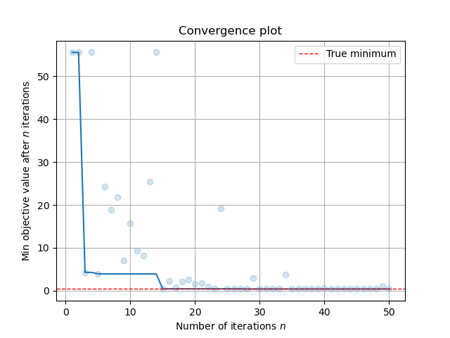
The convergence curve can be plotted for further visualization. If the code is run with Jupyter Notebook, the package HiPlot will show more interesting results:
```python
history.plot_convergence(true_minimum=0.397887)
history.visualize_hiplot()
```
+ Multiple parameter types (FIOC, i.e Float, Integer, Ordinal, and Categorical): input parameters are not limited to float type (real number). For example, the kernel function of Supported Vector Machine is represented by a categorical hyperparameter. Using integer instead of ordinal or categorical type will attach an additional order relationship to parameters, which is not conducive to model optimization.
+ Multi-objective Optimization: Simultaneously optimize multiple different or even conflicting objectives, such as simultaneously optimize the accuracy of the machine learning model and model training/prediction time.
+ Optimization with Constraints: The (black-box) condition should be satisfied while optimizing the objective.
Few existing systems can support the above features at the same time. OpenBox supports not only all the above features but also:
+ Using historical task information to guide the current optimization task, namely transfer learning.
+ Provide parallel optimization algorithm. Support distributed evaluation. Make full use of parallel resources.
+ Multi-fidelity optimization algorithm is provided to further accelerate the search in high evaluation cost scenarios (such as training machine learning models on large datasets).
We will introduce how to use OpenBox in different scenarios in future articles.
### Various Optimization Strategies
OpenBox uses the Bayesian optimization algorithm based on the Random Forest surrogate model by default, which shows outstanding performance on hyperparameter optimization tasks. Compared with the SMAC3 library that uses the same algorithm, OpenBox adopts more optimization strategies, which leads to faster convergence and further improves the performance.
For Bayesian optimization, OpenBox also supports:
+ Gaussian Process surrogate model
+ Tree-structured Parzen Estimator (TPE) model
+ Various acquisition functions, such as EI, PI, LCB, EIC, EHVI, MESMO, USeMO, etc.
Users can choose the optimization strategy based on their needs.
### Usages
Among the existing systems, Google Vizier provides a service for hyperparameter optimization. Unlike the other algorithm libraries, users do not need to deploy the system and run optimization algorithms. They only need to interact with the service to get configuration suggestions, evaluate and update observations. However, Google Vizier is an internal service of Google and is not open-sourced.
Instead, OpenBox provides an online optimization service. Users may deploy the service on their servers using open source code to meet their privacy requirements.
So far, OpenBox supports all the platforms (Linux, macOS, Win10), and there are two ways to use OpenBox: the standalone Python package and distributed BBO service.
+ Standalone Python package: Users can use the black-box optimization algorithm by installing the Python package locally.
+ Distributed BBO service: Users can access the OpenBox service through API, get configuration suggestions from the server, and update observations to the server after evaluating the configuration performance (e.g., training machine learning model and making predictions). Users can monitor and manage the optimization process by visiting the service webpage.
OpenBox is open-source on GitHub: . We welcome more developers to participate in our project.
### Tutorials for Local Usage
In the following, we offer two examples, that is, 1) optimizing mathematical function and 2) tuning hyperparameters of LightGBM, to introduce how to use OpenBox locally. For installation, please refer to our [installation guide](https://open-box.readthedocs.io/en/latest/installation/installation_guide.html).
#### Optimizing Mathematical Function
First, we define the search space and the objective function to be minimized. Here we use the Branin function.
```python
import numpy as np
from openbox import space as sp
# Define Search Space
space = sp.Space()
x1 = sp.Real("x1", -5, 10, default_value=0)
x2 = sp.Real("x2", 0, 15, default_value=0)
space.add_variables([x1, x2])
# Define Objective Function
def branin(config):
x1, x2 = config['x1'], config['x2']
y = (x2-5.1/(4*np.pi**2)*x1**2+5/np.pi*x1-6)**2+10*(1-1/(8*np.pi))*np.cos(x1)+10
return {'objectives': [y]}
```
Next, we call the OpenBox optimization framework Optimizer to perform optimization. Here we set *max_runs*=50, which means that the objective function will be tuned 50 times.
```python
from openbox import Optimizer
opt = Optimizer(branin, space, max_runs=50, task_id='quick_start')
history = opt.run()
```
After optimization, the result is printed as follows:
```python
print(history)
+-------------------------+-------------------+
| Parameters | Optimal Value |
+-------------------------+-------------------+
| x1 | -3.138277 |
| x2 | 12.254526 |
+-------------------------+-------------------+
| Optimal Objective Value | 0.398096578033325 |
+-------------------------+-------------------+
| Num Configs | 50 |
+-------------------------+-------------------+
```
The convergence curve can be plotted for further visualization. If the code is run with Jupyter Notebook, the package HiPlot will show more interesting results:
```python
history.plot_convergence(true_minimum=0.397887)
history.visualize_hiplot()
```
 #### Tuning Hyperparameters of LightGBM
In this example, we define the task using a Python *dictionary*. The most critical part is the definition of the hyperparameter space, that is, the hyperparameters and their corresponding ranges. The following hyperparameter space contains 7 hyperparameters. Another important setting is the number of optimization rounds (*max_runs*). We set it to 100, which means that the objective function will be evaluated 100 times. In other words, the LightGBM model will be tuned 100 times.
```python
config_dict = {
"optimizer": "SMBO",
"parameters": {
"n_estimators": {
"type": "int",
"bound": [100, 1000],
"default": 500,
"q": 50
},
"num_leaves": {
"type": "int",
"bound": [31, 2047],
"default": 128
},
"max_depth": {
"type": "const",
"value": 15
},
"learning_rate": {
"type": "float",
"bound": [1e-3, 0.3],
"default": 0.1,
"log": True
},
"min_child_samples": {
"type": "int",
"bound": [5, 30],
"default": 20
},
"subsample": {
"type": "float",
"bound": [0.7, 1],
"default": 1,
"q": 0.1
},
"colsample_bytree": {
"type": "float",
"bound": [0.7, 1],
"default": 1,
"q": 0.1
},
},
"num_objectives": 1,
"num_constraints": 0,
"max_runs": 100,
"task_id": "tuning_lightgbm"
}
```
Then, we need to define the objective function, which takes the model hyperparameters as inputs and returns the balanced accuracy evaluated using the validation set. Note that:
+ By default, OpenBox **minimizes** the objective function. (If the users want to maximize the objective function, please return its negative value.)
+ To support multiple objectives and constraints, it is recommended to return a Python *dictionary*, and the objectives should be given in a *list* or *tuple*. (Returning a single value is ok if there's only a single objective.)
The following objective function involves two steps: 1) training a LightGBM model on the training set and 2) evaluate its balanced accuracy on the validation set. We directly use the LGBMClassifier provided by the package LightGBM.
```python
from sklearn.model_selection import train_test_split
from sklearn.datasets import load_digits
from sklearn.metrics import balanced_accuracy_score
from lightgbm import LGBMClassifier
# prepare your data
X, y = load_digits(return_X_y=True)
x_train, x_val, y_train, y_val = train_test_split(X, y, test_size=0.2, stratify=y, random_state=1)
def objective_function(config):
# convert Configuration to dict
params = config.get_dictionary().copy()
# fit model
model = LGBMClassifier(**params)
model.fit(x_train, y_train)
# predict and calculate loss
y_pred = model.predict(x_val)
loss = 1 - balanced_accuracy_score(y_val, y_pred) # OpenBox minimizes the objective
# return result dictionary
result = dict(objectives=[loss])
return result
```
After we define the task and the objective function, we use the built-in interface of OpenBox
optimization framework Optimizer to perform optimization.
```python
from openbox import create_optimizer
opt = create_optimizer(objective_function, **config_dict)
history = opt.run()
```
After the optimization, the run history can be printed as follows:
```python
print(history)
+-------------------------+----------------------+
| Parameters | Optimal Value |
+-------------------------+----------------------+
| colsample_bytree | 0.800000 |
| learning_rate | 0.018402 |
| max_depth | 15 |
| min_child_samples | 15 |
| n_estimators | 200 |
| num_leaves | 723 |
| subsample | 0.800000 |
+-------------------------+----------------------+
| Optimal Objective Value | 0.022305877305877297 |
+-------------------------+----------------------+
| Num Configs | 100 |
+-------------------------+----------------------+
```
Similarly, we can plot the convergence curve for further visualization. If the code is run with Jupyter Notebook, the package HiPlot will show more interesting results:
```python
history.plot_convergence()
history.visualize_hiplot()
```
#### Tuning Hyperparameters of LightGBM
In this example, we define the task using a Python *dictionary*. The most critical part is the definition of the hyperparameter space, that is, the hyperparameters and their corresponding ranges. The following hyperparameter space contains 7 hyperparameters. Another important setting is the number of optimization rounds (*max_runs*). We set it to 100, which means that the objective function will be evaluated 100 times. In other words, the LightGBM model will be tuned 100 times.
```python
config_dict = {
"optimizer": "SMBO",
"parameters": {
"n_estimators": {
"type": "int",
"bound": [100, 1000],
"default": 500,
"q": 50
},
"num_leaves": {
"type": "int",
"bound": [31, 2047],
"default": 128
},
"max_depth": {
"type": "const",
"value": 15
},
"learning_rate": {
"type": "float",
"bound": [1e-3, 0.3],
"default": 0.1,
"log": True
},
"min_child_samples": {
"type": "int",
"bound": [5, 30],
"default": 20
},
"subsample": {
"type": "float",
"bound": [0.7, 1],
"default": 1,
"q": 0.1
},
"colsample_bytree": {
"type": "float",
"bound": [0.7, 1],
"default": 1,
"q": 0.1
},
},
"num_objectives": 1,
"num_constraints": 0,
"max_runs": 100,
"task_id": "tuning_lightgbm"
}
```
Then, we need to define the objective function, which takes the model hyperparameters as inputs and returns the balanced accuracy evaluated using the validation set. Note that:
+ By default, OpenBox **minimizes** the objective function. (If the users want to maximize the objective function, please return its negative value.)
+ To support multiple objectives and constraints, it is recommended to return a Python *dictionary*, and the objectives should be given in a *list* or *tuple*. (Returning a single value is ok if there's only a single objective.)
The following objective function involves two steps: 1) training a LightGBM model on the training set and 2) evaluate its balanced accuracy on the validation set. We directly use the LGBMClassifier provided by the package LightGBM.
```python
from sklearn.model_selection import train_test_split
from sklearn.datasets import load_digits
from sklearn.metrics import balanced_accuracy_score
from lightgbm import LGBMClassifier
# prepare your data
X, y = load_digits(return_X_y=True)
x_train, x_val, y_train, y_val = train_test_split(X, y, test_size=0.2, stratify=y, random_state=1)
def objective_function(config):
# convert Configuration to dict
params = config.get_dictionary().copy()
# fit model
model = LGBMClassifier(**params)
model.fit(x_train, y_train)
# predict and calculate loss
y_pred = model.predict(x_val)
loss = 1 - balanced_accuracy_score(y_val, y_pred) # OpenBox minimizes the objective
# return result dictionary
result = dict(objectives=[loss])
return result
```
After we define the task and the objective function, we use the built-in interface of OpenBox
optimization framework Optimizer to perform optimization.
```python
from openbox import create_optimizer
opt = create_optimizer(objective_function, **config_dict)
history = opt.run()
```
After the optimization, the run history can be printed as follows:
```python
print(history)
+-------------------------+----------------------+
| Parameters | Optimal Value |
+-------------------------+----------------------+
| colsample_bytree | 0.800000 |
| learning_rate | 0.018402 |
| max_depth | 15 |
| min_child_samples | 15 |
| n_estimators | 200 |
| num_leaves | 723 |
| subsample | 0.800000 |
+-------------------------+----------------------+
| Optimal Objective Value | 0.022305877305877297 |
+-------------------------+----------------------+
| Num Configs | 100 |
+-------------------------+----------------------+
```
Similarly, we can plot the convergence curve for further visualization. If the code is run with Jupyter Notebook, the package HiPlot will show more interesting results:
```python
history.plot_convergence()
history.visualize_hiplot()
```

 The left figure shows the best observed objective during the optimization while the right figure reflects the relationships between each hyperparameter and the objective.
In addition, Openbox has also integrated the functionality of analyzing hyperparameter importance.
```python
print(history.get_importance())
+-------------------+------------+
| Parameters | Importance |
+-------------------+------------+
| learning_rate | 0.293457 |
| min_child_samples | 0.101243 |
| n_estimators | 0.076895 |
| num_leaves | 0.069107 |
| colsample_bytree | 0.051856 |
| subsample | 0.010067 |
| max_depth | 0.000000 |
+-------------------+------------+
```
In this task, the top-3 influential hyperparameters are *learning_rate*, *min_child_samples*, and *n_estimators*.
In addition, OpenBox supports various scenarios, including multiple objectives, constraints, parallel evaluation, etc. For more characteristics and details about OpenBox, please refer to our [documentation](https://open-box.readthedocs.io).
### Benchmark Results
In this section, we compareOpenBox with other black-box optimization systems on a variety of tasks. Here we display some of the experimental results.
The following figures show the optimality gap of each system over evaluation trials on mathematical problems.
| Ackley-4d | Hartmann-6d |
| :------------------------------: | :------------------------------: |
|  | 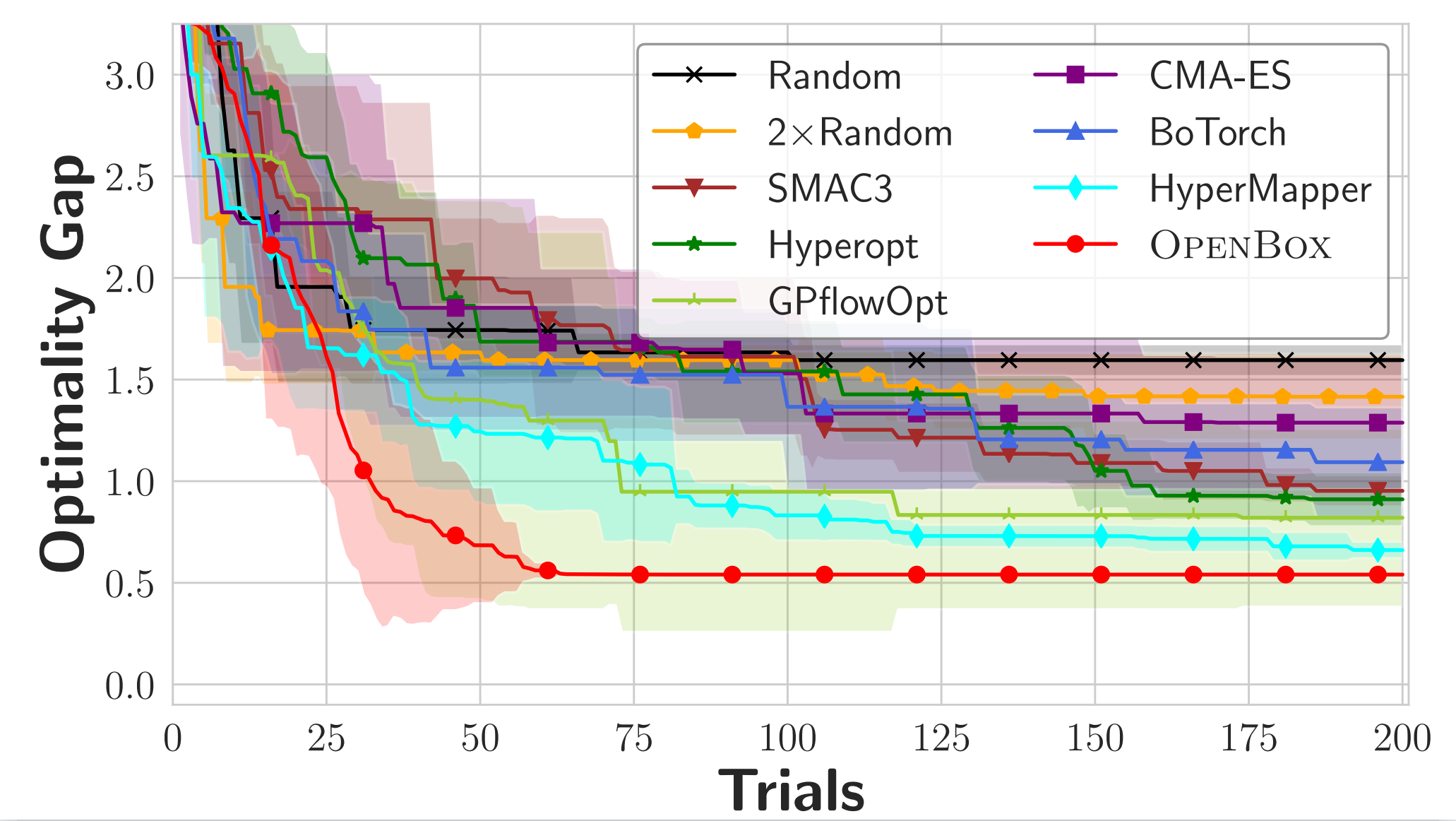 |
We plot the ranks of tuning LightGBM on 25 datasets as follows:
The left figure shows the best observed objective during the optimization while the right figure reflects the relationships between each hyperparameter and the objective.
In addition, Openbox has also integrated the functionality of analyzing hyperparameter importance.
```python
print(history.get_importance())
+-------------------+------------+
| Parameters | Importance |
+-------------------+------------+
| learning_rate | 0.293457 |
| min_child_samples | 0.101243 |
| n_estimators | 0.076895 |
| num_leaves | 0.069107 |
| colsample_bytree | 0.051856 |
| subsample | 0.010067 |
| max_depth | 0.000000 |
+-------------------+------------+
```
In this task, the top-3 influential hyperparameters are *learning_rate*, *min_child_samples*, and *n_estimators*.
In addition, OpenBox supports various scenarios, including multiple objectives, constraints, parallel evaluation, etc. For more characteristics and details about OpenBox, please refer to our [documentation](https://open-box.readthedocs.io).
### Benchmark Results
In this section, we compareOpenBox with other black-box optimization systems on a variety of tasks. Here we display some of the experimental results.
The following figures show the optimality gap of each system over evaluation trials on mathematical problems.
| Ackley-4d | Hartmann-6d |
| :------------------------------: | :------------------------------: |
|  |  |
We plot the ranks of tuning LightGBM on 25 datasets as follows:
 In addition, we compare our transfer learning algorithm with Google Vizier. Before the experiment, we prepare 25 datasets and the corresponding tuning history on each dataset. The experiment is conducted in a ''leave-one-out'' fashion, which means we tune on one dataset again while using the history of the remaining 24 datasets. The average ranks over evaluation trials are as follows: (SMAC3 is the baseline without using transfer learning)
 We can have that, OpenBox outperforms the existing black-box optimization systems.
## Summary
In this article, we introduced the black-box optimization problem and our open source black-box optimization system [OpenBox](). We are actively accepting code contributions to the OpenBox project.
In the future, we will continue to introduce more usages of OpenBox, including the deployment of online service, parallel evaluation, multi-fidelity optimization, etc.
## Reference
[1]
We can have that, OpenBox outperforms the existing black-box optimization systems.
## Summary
In this article, we introduced the black-box optimization problem and our open source black-box optimization system [OpenBox](). We are actively accepting code contributions to the OpenBox project.
In the future, we will continue to introduce more usages of OpenBox, including the deployment of online service, parallel evaluation, multi-fidelity optimization, etc.
## Reference
[1]